Posts

SQL Joins: INNER, LEFT, RIGHT, FULL

Image
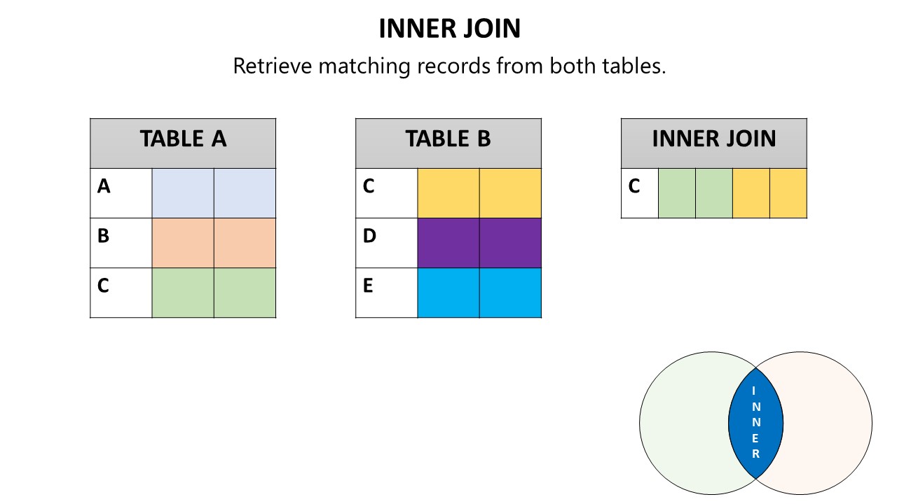
As a data analyst, you’ll often encounter situations where you need to combine data from different tables. SQL joins are the tools that allow you to do just that. SQL joins are a fundamental concept for data analysts. Understanding SQL joins is essential for manipulating relational databases effectively and extracting meaningful information from disparate datasets. In this blog post, we'll explore the different types of SQL joins i.e. inner join, left join, right join, full join. Why Learn SQL Joins? SQL joins are like puzzle pieces that fit together to create a complete picture. Here’s why they matter: Data Integration : Combine related data from different tables. Holistic Insights : Uncover patterns and relationships across datasets. Efficient Queries : Optimize data retrieval by fetching only the necessary information. Types of SQL Joins 1. INNER JOIN (or JOIN) Purpose : Returns rows when there is at least one match in both tables based on the join condition. This is the most co...

XLOOKUP Function in Excel

Image
In our previous blog post we have already learned about 2 most useful lookup functions: VLOOKUP and HLOOKUP . In this blog post, we’ll explore what XLOOKUP is, its syntax, why you should use it, its pros and cons, and provide some practical examples. The  XLOOKUP  function revolutionize the way we search and retrieve data. XLOOKUP function is a modern and versatile replacement for traditional lookup functions in Excel. It allows you to find things in a table or range by row, regardless of whether the return column is on the left or right side. It’s like a search engine for your Excel data. Here’s what you need to know: Syntax : =XLOOKUP(lookup_value, lookup_array, return_array, [if_not_found], [match_mode], [search_mode]) Arguments : lookup_value : The value you want to search for. lookup_array : The range or array to search. return_array : The range or array from which to return results. [ if_not_found ] : (Optional) Specify what to return if no match is found. [ match_...

HLOOKUP Function in Excel

Image
In the previous blog post we learned about VLOOKUP function in Excel . In this blog post, we will explain how the HLOOKUP function works, what its syntax is, what are its advantages and limitations, and how to use it with some examples.  HLOOKUP stands for horizontal lookup and it allows you to search for a value in the first row of a table and return a value from the same column in another row. The syntax of the HLOOKUP function is: =HLOOKUP(lookup_value, table_array, row_index_num, [range_lookup]) The arguments of the function are: lookup_value : The value that you want to find in the first row of the table. This can be a number, text, logical value, or a cell reference. table_array : The range of cells that contains the table or array of data. The first row of this range should contain the lookup values. row_index_num : The row number in the table from which you want to return a value. This can be a positive integer or a cell reference. [range_lookup] : (Optional argument) ...

VLOOKUP function to perform lookups in Excel

Image
In this blog post, we will explore VLOOKUP function in Excel, and see how they can help you find the information you need. The VLOOKUP function is one of the most basic and widely used lookup functions in Excel. It allows you to search for a value in the first column of a table, and return a value from another column in the same row. The syntax of the VLOOKUP function is: =VLOOKUP(lookup_value, table_array, col_index_num, [range_lookup]) The arguments of the VLOOKUP function are: Table Argument Explanation lookup_value The value that you want to find in the first column of the table. This can be a cell reference, a text, a number, or a logical value. table_array The range of cells that contains the table of data. The first column of this range should contain the lookup value, and other columns should contain the return values. col_index_num The column ...

Logical Functions in Excel (IF, AND, OR, XOR, IFERROR, IFNA, IFS, and SWITCH)

Image
Logical functions are functions that allow you to test conditions and return values based on the results. In this blog post, we will learn how to use nine common logical functions in Excel: IF, AND, OR, XOR, NOT, IFERROR, IFNA, IFS, and SWITCH.  IF Function The IF function allows you to make decisions based on whether a condition is true or false. The IF function can also be nested inside another IF function, to test multiple conditions and return different values.  Syntax of the IF function is: =IF(logical_test, value_if_true, value_if_false) Student Data Example I have also applied conditional formatting for cells containing "F" values AND Function The AND function checks multiple conditions and returns TRUE if all of them are true , and FALSE if any of them are false. You can have up to 255 conditions in the AND function.  Syntax of the AND function is: =AND(condition1, condition2, …)  Employee Data Example OR Function The OR function checks multiple conditions an...

Introduction to Pivot Table in Excel - Advanced

Image
In the previous blog post, we learned the  Basics of Pivot Table  in Excel. In this blog post, we will explore some of the advanced features of pivot tables, such as slicers, timelines, calculated fields, pivot charts, managing relationships, etc. These features can help you change your existing pivot table and create different views of your data every time. Slicers Slicers are used to filter your data by selecting specific values from a field. For example in this data table , we have a column named Product (Crayons, Geometry Box, Paper, Pen, Stapler, Sticky Notes)  you can use a slicer to show only the data for a particular product or products.  Steps to add a Slicer: Select your pivot table ➡️ PivotTable Analyze ➡️ Click on "Insert Slicer" ➡️Choose the field for the slicer. A slicer window will appear, where you can select a field and a slicer will be inserted. You can select one option or multiselect by holding down the CTRL key while making your selections. You c...

Introduction to Pivot Table in Excel - Basics

Image
Pivot tables are one of the most powerful and useful features in Excel. Allowing us to quickly summarize, analyze, and explore large amounts of data in various ways. It is a special type of table that displays the summary of a data set and helps us in analyzing the data in seconds without knowing any formulas and functions. It consists of four areas: rows, columns, values, and filters. You can drag and drop different fields from your data set into these areas to create different views of your data. In this blog post, we will introduce the basics of pivot tables. Converting data to tabular data before inserting Pivot Table is an added advantage as this eliminates the need to frequently adjust the table range as new entries are added (select a cell from the data and click CTRL+T and then OK).  Additionally the following conditions need to be fulfilled: ✔ Each column should have unique headers, and the headers should be descriptive enough.       For ex. If Revenue...